Binomial Logistic Regression
About
Logistic regression models are one of the most common machine learning models for handling classification problems. Binomial Logistic Regression is just one type of logistic regression model. It refers to the classification of two variables where a probability is used to determine a binary outcome, hence the “bi” in “binomial.” The outcome is either True or False—0 or 1.
An example of binomial logistic regression is predicting the likelihood of COVID-19 within a population. A person either has COVID-19 or they don’t, and a threshold must be established to distinguish these results as accurately as possible.
Sigmoid Function
These predictions are not fit to a line, as is the case with linear regression models. Instead, logistic regression models are fit to a sigmoid function, shown to the right.
Sigmoid functions can be modelled using the following equation: $\large{f(x) = \frac{1}{1 + e^{-y}}}$
For each $x$, the resulting $y$ value represents the probability that a result is True. In the COVID-19 example, this represents how confident a doctor is that a person has contracted the virus. In the picture to the right, negative results are blue and positive results are red.
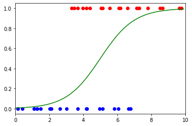
Image by Author
The Process
To do binomial logistic regression, we will need to do a variety of things:
-
Create a training dataset.
-
Use PyTorch to create our model.
-
Fit our data to the model.
The first step of our logistic regression problem is to create the training datset. First, we should set a seed to ensure the reproducibility of our random data.
import numpy as np
import matplotlib.pyplot as plt
import torch
import torch.nn as nn
from torch.nn import Linear

torch.manual_seed(42)   # set a random seed
We must use a linear model from PyTorch because we are dealing with one
input, $x$, and one output, $y$. Therefore, our model is linear. To do
this, we will use PyTorch’s Linear function:
model = Linear(in_features=1, out_features=1) # use a linear model
Next, we must generate our blue X and red X data, making sure to reshape them from a row vector to a column vector. The blue ones will be between 0 and 7, and the red ones will be between 7 and 10. For the $y$ values, the blue points represent a negative COVID-19 test, so they will all be
- For the red points, they represent a positive COVID-19 test, so they will be 1. Below is the code and its output:
blue_x = (torch.rand(20) * 7).reshape(-1,1)   # random floats between 0 and 7
blue_y = torch.zeros(20).reshape(-1,1)

red_x = (torch.rand(20) * 7+3).reshape(-1,1)  # random floats between 3 and 10
red_y = torch.ones(20).reshape(-1,1)

X = torch.vstack([blue_x, red_x])   # matrix of x values
Y = torch.vstack([blue_y, red_y])   # matrix of y values
Now, our code should look like this:
import numpy as np
import matplotlib.pyplot as plt
import torch
import torch.nn as nn
from torch.nn import Linear

torch.manual_seed(42)   # set a random seed

model = Linear(in_features=1, out_features=1) # use a linear model

blue_x = (torch.rand(20) * 7).reshape(-1,1)   # random floats between 0 and 7
blue_y = torch.zeros(20).reshape(-1,1)

red_x = (torch.rand(20) * 7+3).reshape(-1,1)  # random floats between 3 and 10
red_y = torch.ones(20).reshape(-1,1)

X = torch.vstack([blue_x, red_x])   # matrix of x values
Y = torch.vstack([blue_y, red_y])   # matrix of y values
Optimization
We will be using the process of gradient descent to optimize the loss of our sigmoid function. The loss is calculated based on how well the function fits the data, which is governed by the slope and intercept of the sigmoid curve. We need gradient descent to find the optimal slope and intercept.
We will also use Binary Cross Entropy (BCE) as our loss function, or the log loss function. For logistic regression in general, loss functions that do not incorporate logrithms will not work.
To implement BCE as our loss function, we will set this up as our criterion, and Stochastic Gradient Descent as our means of optimizing it. Since this is the function we’ll be optimizing, we need to pass in the model parameters and a learning rate.
epochs = 2000   # run 2000 iterations
criterion = nn.BCELoss()    # implement binary cross entropy loss function

optimizer = torch.optim.SGD(model.parameters(), lr = .1) # stochastic gradient descent
Now, we are ready to start gradient descent to optimize our loss. We must zero out the gradient, find the $\hat{y}$ value by plugging our data into the sigmoid function, calculate the loss, and find the gradient of the loss function. Then, we must make a step, making sure to store our new slope and intercept for the next iteration.
optimizer.zero_grad()
Yhat = torch.sigmoid(model(X))
loss = criterion(Yhat,Y)
loss.backward()
optimizer.step()
Finishing Up
To find the optimal slope and intercept, we are essentially training our model. We must apply gradient descent for a number of iterations, or epochs. In this example, we’ll use 2,000 epochs to demonstrate.
epochs = 2000   # run 2000 iterations
criterion = nn.BCELoss()    # implement binary cross entropy loss function

optimizer = torch.optim.SGD(model.parameters(), lr = .1) # stochastic gradient descent

for i in range(epochs):
    optimizer.zero_grad()
    Yhat = torch.sigmoid(model(X))
    loss = criterion(Yhat,Y)
    loss.backward()
    optimizer.step()

    print(f"epoch: {i+1}")
    print(f"loss: {loss: .5f}")
    print(f"slope: {model.weight.item(): .5f}")
    print(f"intercept: {model.bias.item(): .5f}")
    print()
Putting all of the code pieces together, we should get the following code:
import numpy as np
import matplotlib.pyplot as plt
import torch
import torch.nn as nn
from torch.nn import Linear

torch.manual_seed(42)   # set a random seed

model = Linear(in_features=1, out_features=1) # use a linear model

blue_x = (torch.rand(20) * 7).reshape(-1,1)   # random floats between 0 and 7
blue_y = torch.zeros(20).reshape(-1,1)

red_x = (torch.rand(20) * 7+3).reshape(-1,1)  # random floats between 3 and 10
red_y = torch.ones(20).reshape(-1,1)

X = torch.vstack([blue_x, red_x])   # matrix of x values
Y = torch.vstack([blue_y, red_y])   # matrix of y values

epochs = 2000   # run 2000 iterations
criterion = nn.BCELoss()    # implement binary cross entropy loss function

optimizer = torch.optim.SGD(model.parameters(), lr = .1) # stochastic gradient descent

for i in range(epochs):
    optimizer.zero_grad()
    Yhat = torch.sigmoid(model(X))
    loss = criterion(Yhat,Y)
    loss.backward()
    optimizer.step()

    print(f"epoch: {i+1}")
    print(f"loss: {loss: .5f}")
    print(f"slope: {model.weight.item(): .5f}")
    print(f"intercept: {model.bias.item(): .5f}")
    print()
Final output after two thousand epochs:
epoch: 2000
loss:  0.53861
slope:  0.61276
intercept: -3.17314
Visualization
And finally, we can plot the data along with the sigmoid function to get the following visualization:
x = np.arange(0,10,.1)
y = model.weight.item()*x + model.bias.item()

plt.plot(x, 1/(1 + np.exp(-y)), color="green")

plt.xlim(0,10)
plt.scatter(blue_x, blue_y, color="blue")
plt.scatter(red_x, red_y, color="red")

plt.show()
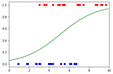
Image by Author
Limitations
One of the biggest problems with binary classification is the need for a threshold. In the case of logistic regression, this threshold should be at the value of $x$ where $y$ is at 50%. The question we’re trying to answer is where to put the threshold?
In the case of COVID-19 testing, the original example illustrates this dilemma. If we put our threshold at $x=5$, we can clearly see blue dots that should be red, and red dots that should be blue.
The overhanging red dots are called false positives—areas in which the model incorrectly predicted the positive class. The overhanging blue dots are called false negatives—areas in which the model incorrectly predicted the negative class.
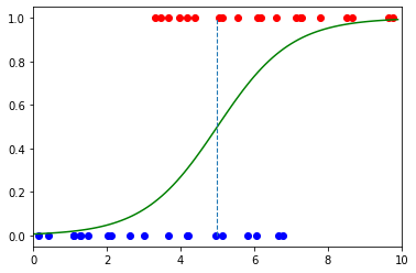
Image by Author
Conclusion
A successful binomial logistic regression model will have reduced the amount of false negatives, as these often cause the most danger. Having COVID-19 but testing negative is a serious risk to the health and safety of others.
By using Binomial Logistic Regression on the data available, we can determine the optimal place to put our threshold, and thus help to reduce uncertainty and make more informed decisions.