Multinominal Logistic Regression
Multinomial logistic regression is a statistical method used for predicting categorical outcomes with more than two categories. It is particularly useful when the dependent variable is categorical rather than continuous.
Categorical Predictions
In multinomial logistic regression, the model predicts the probabilities of an observation belonging to each category of the dependent variable. These probabilities can be interpreted as the likelihood of the observation falling into each category. The predicted category is typically the one with the highest probability, making it a categorical prediction rather than a continuous one.
In contrast, standard logistic regression, also known as binary logistic regression—a special case of Binomial Logistic Regression—is used when the dependent variable has two categories only. It predicts the probability of an observation belonging to one category versus another. The predictions in binary logistic regression are continuous probabilities between 0 and 1.
Under the Hood
Below is the mathematics behind multinomial logistic regression. These equations represent a set of log-linear models, where the logarithm of the ratio of the probabilities of each class is linearly related to a predictor variable $X_i$ through a coefficient (or slope) parameter, denoted by $\beta_1$, $\beta_2$, …, $\beta_{K-1}$. The notation $\text{P}(Y_i = K)$ represents the probability of observation $i$ belonging to class $K$, where $K$ is an integer representation of each class, starting at 1.
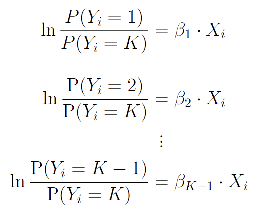
Image by Author
From these equations, we can simplify to the ones below, which are alternate forms of the equations we saw earlier. They are derived from the fact that the probabilities of all $K$ classes must sum to 1. In these equations, $\text{P}(Y_i = K)$ is used as a reference category, and the probabilities of the other $K-1$ categories are expressed relative to this reference category using exponential functions of the predictor variable $X_i$ and the corresponding coefficient $\beta_K$.
The exponential function $e$ in these equations is used to transform the linear predictor (i.e., $\beta_K \cdot X_i$) into a probability, which is always positive and bounded between 0 and 1. By applying the exponential function $e$ to both sides of the previous equations, we get the following for the first class:
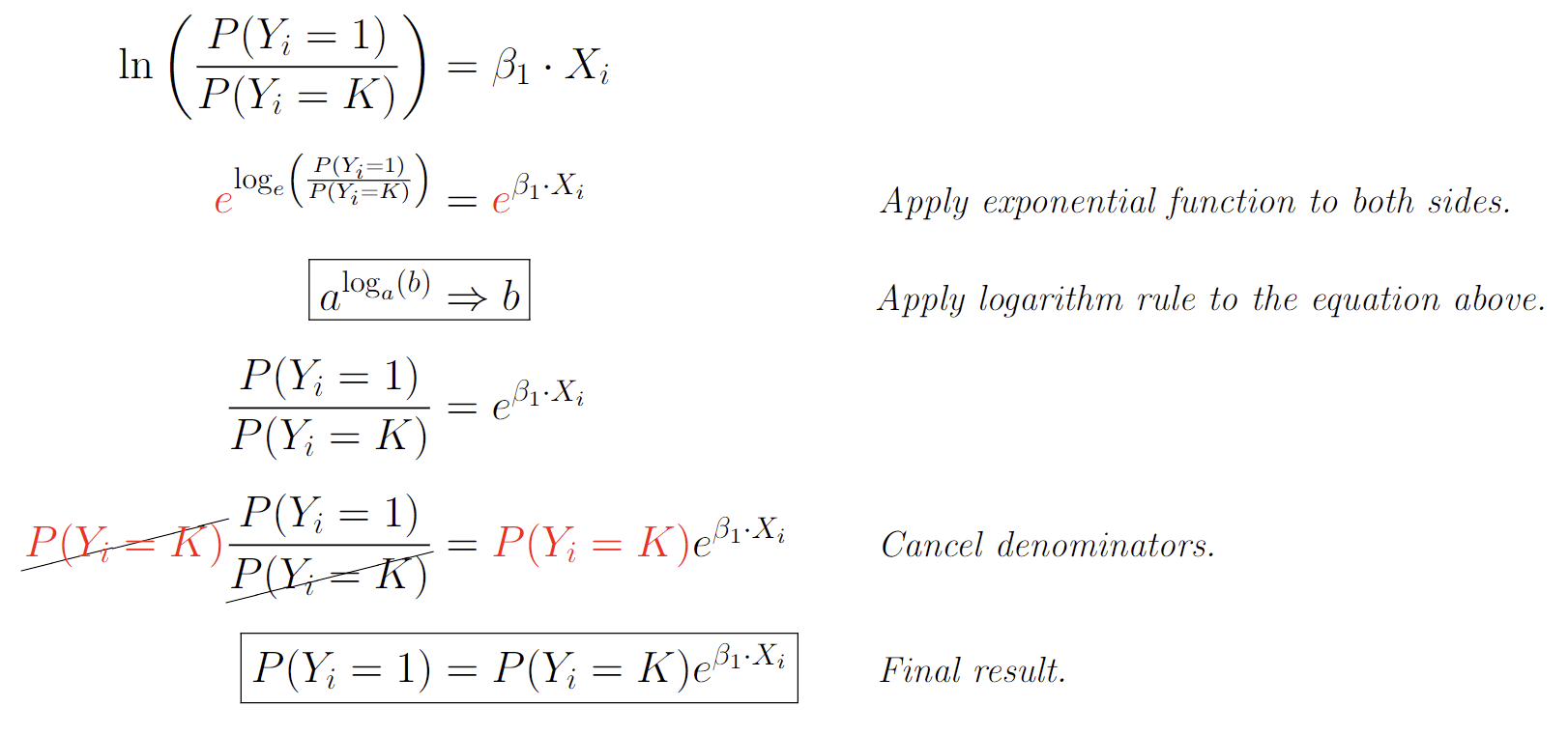
Image by Author
These equations are often used in the context of multinomial logistic regression, where the goal is to predict the probability of an observation belonging to each of $K$ classes based on one or more predictor variables.
About the Data
In this example, we will be using University of California, Irvine’s abalone dataset to predict the gender of an abalone. A multivariate linear regression model can be used to predict the age, though for this example, we are predicting the gender of a given abalone based on several distinct features.
Using the Python pandas package, we can see the shape of the data, as well as the first few rows.
import pandas as pd

df = pd.read_csv("https://raw.githubusercontent.com/s-lasch/CIS-280/main/abalone.csv")    # read csv
df.shape    # get shape
(4177, 9)
df.head() # show first 5 rows
| sex   | length | diameter | height | whole_weight | shucked_weight | viscera_weight | shell_weight | rings |
--------------------------------------------------------------------------------------------------------------
| M	| 0.455  | 0.365    | 0.095  | 0.5140       | 0.2245         | 0.1010         | 0.150        | 15    |
| M	| 0.350  | 0.265    | 0.090  | 0.2255       | 0.0995         | 0.0485         | 0.070        | 7     |
| F	| 0.530  | 0.420    | 0.135  | 0.6770       | 0.2565         | 0.1415         | 0.210        | 9     |
| M	| 0.440  | 0.365    | 0.125  | 0.5160       | 0.2155         | 0.1140         | 0.155        | 10    |
| I	| 0.330  | 0.255    | 0.080  | 0.2050       | 0.0895         | 0.0395         | 0.055        | 7     |
Processing the Data
We can see that there are three distinct classes—or categories—in the sex column: M, F, and I, which stand for Male, Female, and Infant. These represent the classes that our model is going to predict based on the other columns in the dataset.
df['sex'].value_counts().sort_values(ascending=False) # count the number of distinct classes
M    1528
I    1342
F    1307
Name: sex, dtype: int64
This means our $y$ data will be the sex column, and our $X$ data will be all columns except for sex.
X = df.drop(['sex'], axis=1)
y = df['sex']
Now we are ready to split the data into training versus testing. We can do this using the scikitlearn package as used below:
from sklearn.model_selection import train_test_split

X_train, X_test, y_train, y_test = train_test_split(X, y, test_size = 0.20, random_state = 5)

print(X_train.shape)
print(X_test.shape)
print(y_train.shape)
print(y_test.shape)
(3341, 8)
(836, 8)
(3341,)
(836,)
One-Hot Encoding
Now that we have our training and testing data, it is important to remember that any regression model expects either integer or float inputs. Because the sex column is categorical, we need to apply integer encoding to use them for regression. For this, we will apply one-hot encoding, which will assign an integer to each distinct class.
y_train = y_train.apply(lambda x: 0 if x == "M" else 1 if x == "F" else 2)
y_test = y_test.apply(lambda x: 0 if x == "M" else 1 if x == "F" else 2)
Now that the $y$ data is encoded, we have to convert each of the train/test datasets to a torch.tensor. This is crucial for any regression using Pytorch, as it can only take tensors.
X_train_tensor = torch.tensor(X_train.to_numpy()).float()
X_test_tensor = torch.tensor(X_test.to_numpy()).float()
y_train_tensor = torch.tensor(y_train.to_numpy()).long()
y_test_tensor = torch.tensor(y_test.to_numpy()).long()
For more information on tensors, a really in-depth resource can be found here.
The Model
With the data processing complete, we can now begin the process of creating the model. For the implementation of this model, we will be using Pytorch library. Since there are 8 features used to determine the sex, we need to set the in_features to 8. Since the model can only predict three possible classes, out_features will be set to 3. For more information on Pytorch’s torch.nn module, refer to the documentation.
import torch
import torch.nn as nn
from torch.nn import Linear
import torch.nn.functional as F


torch.manual_seed(348965)                                 # keep random values consistent

model = Linear(in_features=8, out_features=3)             # define the model

# define the loss function and optimizer
criterion = nn.CrossEntropyLoss()                         # use cross-entropy loss for multi-class classification
optimizer = torch.optim.SGD(model.parameters(), lr=.01)   # learning rate of 0.01, and Stocastic Gradient descent optimizer
Training the Model
num_epochs = 2500    # loop iterations

for epoch in range(num_epochs):
    # forward pass
    outputs = model(X_train_tensor)
    loss = criterion(outputs, y_train_tensor)

    # backward and optimize
    optimizer.zero_grad()
    loss.backward()
    optimizer.step()

    # print progress every 100 epochs
    if (epoch+1) % 100 == 0:
        print('Epoch [{}/{}]\tLoss: {:.4f}'.format(epoch+1, num_epochs, loss.item()))
Epoch [100/2500]     Loss: 1.1178
Epoch [200/2500]     Loss: 1.1006
Epoch [300/2500]     Loss: 1.0850
Epoch [400/2500]     Loss: 1.0708
Epoch [500/2500]     Loss: 1.0579
Epoch [600/2500]     Loss: 1.0460
Epoch [700/2500]     Loss: 1.0352
Epoch [800/2500]     Loss: 1.0252
Epoch [900/2500]     Loss: 1.0161
Epoch [1000/2500]    Loss: 1.0077
Epoch [1100/2500]    Loss: 0.9999
Epoch [1200/2500]    Loss: 0.9927
Epoch [1300/2500]    Loss: 0.9860
Epoch [1400/2500]    Loss: 0.9799
Epoch [1500/2500]    Loss: 0.9741
Epoch [1600/2500]    Loss: 0.9688
Epoch [1700/2500]    Loss: 0.9638
Epoch [1800/2500]    Loss: 0.9592
Epoch [1900/2500]    Loss: 0.9549
Epoch [2000/2500]    Loss: 0.9509
Epoch [2100/2500]    Loss: 0.9471
Epoch [2200/2500]    Loss: 0.9435
Epoch [2300/2500]    Loss: 0.9402
Epoch [2400/2500]    Loss: 0.9371
Epoch [2500/2500]    Loss: 0.9342
Validation
Now to check the accuracy, we can run the following code:
outputs = model(X_test_tensor)
_, preds = torch.max(outputs, dim=1)
accuracy = torch.mean((preds == y_test_tensor).float())
print('\nAccuracy: {:.2f}%'.format(accuracy.item()*100))
Accuracy: 52.63%
This means that our model accurately identified the gender of abalone based on 8 distinct features 53% of the time.
Complete Code
Here is the complete code:
import torch
import torch.nn as nn
from torch.nn import Linear
import torch.nn.functional as F


torch.manual_seed(348965)                                 # keep random values consistent

model = Linear(in_features=8, out_features=3)             # define the model

# define the loss function and optimizer
criterion = nn.CrossEntropyLoss()                         # use cross-entropy loss for multi-class classification
optimizer = torch.optim.SGD(model.parameters(), lr=.01)   # learning rate of 0.01, and Stocastic Gradient descent optimizer

# convert the data to PyTorch tensors
X_train_tensor = torch.tensor(X_train.to_numpy()).float()
X_test_tensor = torch.tensor(X_test.to_numpy()).float()
y_train_tensor = torch.tensor(y_train.to_numpy()).long()
y_test_tensor = torch.tensor(y_test.to_numpy()).long()

# train the model
num_epochs = 2500    # loop iterations

for epoch in range(num_epochs):
    # forward pass
    outputs = model(X_train_tensor)
    loss = criterion(outputs, y_train_tensor)

    # backward and optimize
    optimizer.zero_grad()
    loss.backward()
    optimizer.step()

    # print progress every 100 epochs
    if (epoch+1) % 100 == 0:
        print('Epoch [{}/{}]\tLoss: {:.4f}'.format(epoch+1, num_epochs, loss.item()))


outputs = model(X_test_tensor)
_, preds = torch.max(outputs, dim=1)
accuracy = torch.mean((preds == y_test_tensor).float())
print('\nAccuracy: {:.2f}%'.format(accuracy.item()*100))
Epoch [100/2500]	   Loss: 1.1178
Epoch [200/2500]	   Loss: 1.1006
Epoch [300/2500]	   Loss: 1.0850
Epoch [400/2500]	   Loss: 1.0708
Epoch [500/2500]	   Loss: 1.0579
Epoch [600/2500]	   Loss: 1.0460
Epoch [700/2500]	   Loss: 1.0352
Epoch [800/2500]	   Loss: 1.0252
Epoch [900/2500]	   Loss: 1.0161
Epoch [1000/2500]	   Loss: 1.0077
Epoch [1100/2500]	   Loss: 0.9999
Epoch [1200/2500]	   Loss: 0.9927
Epoch [1300/2500]	   Loss: 0.9860
Epoch [1400/2500]	   Loss: 0.9799
Epoch [1500/2500]	   Loss: 0.9741
Epoch [1600/2500]	   Loss: 0.9688
Epoch [1700/2500]	   Loss: 0.9638
Epoch [1800/2500]	   Loss: 0.9592
Epoch [1900/2500]	   Loss: 0.9549
Epoch [2000/2500]	   Loss: 0.9509
Epoch [2100/2500]	   Loss: 0.9471
Epoch [2200/2500]	   Loss: 0.9435
Epoch [2300/2500]	   Loss: 0.9402
Epoch [2400/2500]	   Loss: 0.9371
Epoch [2500/2500]	   Loss: 0.9342

Accuracy: 52.63%